Showing posts with label finance. Show all posts

Happy 20th Anniversary !

Happy 20th Anniversary of Stock Market Crash 1997

In financial markets, Black Monday is the name given to Monday, October 19, 1987, when the Dow Jones Industrial Average (DJIA) dropped by 508 points to 1739 (22.6%),[1] and on which similar enormous drops occurred across the world. By the end of October, stock markets in Hong Kong had fallen 45.8%, Australia 41.8%, Spain 31%, the United Kingdom 26.4%, the United States 22.68%, and Canada 22.5%. (The terms Black Monday and Black Tuesday are also applied to October 28 and 29, 1929, which occurred after Black Thursday on October 24, which started the Stock Market Crash of 1929.)
(read more)

Konstruksi portfolio reksa dana Indonesia

Cuma suatu usulan.

Suatu portfolio investasi dapat direalisasikan cukup dengan menggabungkan beberapa reksa dana ke dlm suatu portfolio setting yang dikonstruksikan sesuai dengan risk profile investor. Logikanya adalah reksa dana itu sendiri sudah merupakan suatu portfolio terdiri dari beberapa saham dan/atau obligasi.

Kelemahan reksa dana di Indonesia adalah pengkategoriannya yang masih umum sbb: reksa dana saham, fixed income, campuran, pasar uang dan indeks. Idealnya bagi investor di Indonesia, mereka paling tidak harus mampu membedakan reksa dana mana yang berada dlm konteks Indonesia, negara2 berkembang lainnya dan negara2 maju spt Australia, US, Jepang dan US. Pasar modal tiap negara atau regional pada kenyataannya memiliki tingkat return dan risiko yang berbeda. Dengan demikian, konstruksi portfolio bisa dibangun sesuai dengan profil risiko masing2 klien.

Risk profile seorang investor dapat dikategorikan sbb: defensive, conservative, balanced, growth dan aggressive. Sementara pembagian kelas asset dapat dipisahakan menjadi income asset dan growth asset. Income asset terdiri dari cash dan fixed income (obligasi). Growth asset terdiri dari: property dan shares (saham).

Berkaitan dengan profil risiko, biasanya orang muda memiliki risk profile growth dan aggressive dan orang tua cenderung balanced, conservative dan defensive. Rangka waktu (jangka pendek atau jangka panjang), toleransi return dan tujuan keuangan juga menentukan risk profile seseorang.

Ringkasan kategori asset dalam portfolio yang disusun berdasarkan tingkat return dan risiko adalah sbb:

Income asset:
1. cash: deposito US Dollar
2. cash: deposito Rupiah
3. reksa dana fixed income negara maju: Australia, US, Eropa, Japan, Singapore, HK
4. reksa dana fixed income Asia: China, Taiwan, Korea, Malaysia
5. reksa dana fixed income Indonesia

Growth asset:
6. reksa dana properti Indonesia
7. reksa dana saham negara maju: Australia, US, Eropa, Japan, Singapore, HK
8. reksa dana saham Asia: China, Taiwan Korea, Malaysia
9. reksa dana saham Indonesia

Reksa dana 9 menunjukkan investasi yang paling tinggi tingkat risikonya, tapi paling tinggi juga tingkat returnnya. Pembagian ini mungkin akan didukung para ekonom krn memang kenyataannya demikian. Investasi property di Indonesia mungkin bisa didebatkan lebih berisiko dari pada investasi saham negara maju.

Untuk penyelidikan lebih lanjut, silakan kunjungi website MSCI-Barra untuk melihat tingkat return per negara atau regional.

Usulan konstruksi portfolio

Usulan konstruksi portfolio ini dibuat berdasarkan pengalokasian strategis (strategic asset allocation) dan masih dapat dimodifikasi dalam pengalokasian teknis (technical asset allocation) sesuai dengan kondisi pasar modal domestik dan internasional serta kecenderungan kurs Rupiah terhadap mata uang asing.


Defensive Portfolio

Income asset: 90%
1. deposito USD = 5%
2. deposito IDR = 5%
3. RD fixed income negara maju = 40%
4. RD fixed income Asia = 20%
5. RD fixed income Indonesia = 20%

Growth asset: 10%
6. RD properti Indonesia = 5%
7. RD saham negara maju = 5%
8. RD saham Asia = 0%
9. RD saham Indonesia = 0%


Conservative Portfolio

Income asset: 70%
1. deposito USD = 3%
2. deposito IDR = 2%
3. RD fixed income negara maju = 25%
4. RD fixed income Asia = 20%
5. RD fixed income Indonesia = 20%

Growth asset: 30%
6. RD properti Indonesia = 10%
7. RD saham negara maju = 10%
8. RD saham Asia = 5%
9. RD saham Indonesia = 5%


Balanced Portfolio

Income asset: 50%
1. deposito USD = 0%
2. deposito IDR = 5%
3. RD fixed income negara maju = 15%
4. RD fixed income Asia = 15%
5. RD fixed income Indonesia = 15%

Growth asset: 50%
6. RD properti Indonesia = 10%
7. RD saham negara maju = 20%
8. RD saham Asia = 10%
9. RD saham Indonesia = 10%


Growth Portfolio

Income asset: 30%
1. deposito USD = 0%
2. deposito IDR = 5%
3. RD fixed income negara maju = 5%
4. RD fixed income Asia = 5%
5. RD fixed income Indonesia = 15%

Growth asset: 70%
6. RD properti Indonesia = 15%
7. RD saham negara maju = 15%
8. RD saham Asia = 15%
9. RD saham Indonesia = 25%


Aggressive Portfolio

Income asset: 10%
1. deposito USD = 0%
2. deposito IDR = 0%
3. RD fixed income negara maju = 0%
4. RD fixed income Asia = 5%
5. RD fixed income Indonesia = 5%

Growth asset: 90%
6. RD properti Indonesia = 15%
7. RD saham negara maju = 20%
8. RD saham Asia = 25%
9. RD saham Indonesia = 30%


Ketersediaan reksa dana macam ini

Mungkin ketersediaan reksa dana macam ini masih menjadi isu utama di bisnis reksa dana Indonesia. Namun, saya yakin peningkatan pengetahuan investasi kelas menengah Indonesia akan mendorong manajer investasi yang berdomisili di Indonesia untuk menciptakan produk reksa dana yang lebih kreatif dan menunjang pembentukan model portfolio di masa mendatang.

Daftar lengkap reksa dana Indonesia dapat ditemui di website Bapepam.

Update 1

Baru mendapat konfirmasi dari John D Item, CFA bahwa:

Industri reksadana saat ini hanya boleh investasi instrumen luar negeri maksimum 15% dari total portofolio. Oleh karena itu, penggunaan reksadana lokal untuk analisa alokasi aset domestik maupun internasional saat ini belum relevan.


Kalau begitu, kreatifitas manajer investasi lokal masih terbatas dan reksa dana asing (yang dikelola manajer investasi Singapore misalnya) mungkin masih belum boleh dijual di Indonesia.

Hal ini memberi kesan bahwa portfolio investasi reksa dana di Indonesia pada dasarnya aggressive, atau paling tidak growth atau balanced. Bagaimana nasib para orang tua dengan portfolio defensive atau conservative?


Update 2

Ada pertanyaan kritis yg bagus dari Bahar, Indonesian hedge fund manager yg berdomisili di Singapur, di blog-nya. Kenapa di blog-nya? Krn saya me-link post ini ke comment-nya. Fair enough :)

Pertanyaannya:
Angka2 yang muncul di ” konstruksi portfolio RD Indonesia” berdasarkan apa bung Anymatters? Some Markowitz based optimisation?


Jawaban saya:
thanks bung iHedge. keliatannya Prof Roger Ibbotson dr Morningstar yg mengembangkan model alokasi aset itu msh berkiblat ke teori Markowitz deh.

angka2 itu saya ambil dr model portfolio-nya Morningstar NZ yg didistribusikan ke fin adviser (maaf hasil risetnya tdk bisa dishare) dan saya modifikasi sendiri sesuai dgn situasi Indonesia. dimana komponen asset class-nya saya rate berdasarkan tingkat return indeks per negara/regional di website MSCI-Barra.

proporsi asset class antara income-growth menggunakan alokasi aset strategik (blm taktikal), yaitu defensive (90-10), conservative (70-30), balanced (50-50), growth (30-70) dan aggressive (30-70).

mengenai produk2 apa saja dlm komponen asset class tsb, saya belum bisa recommend. mungkin nanti kalo pulang ke Jkt, bisa buat ide usaha :)

tapi kalo ada waktu, saya mau riset produk2 RD yg di-archive di website Bapepam. kalo ada waktu.

mungkin Morningstar Singapore sdh watch RD Indonesia dan memiliki konstruksi model portfolio RD di Indonesia. cek aja, alamatnya 80 Raffles Place, Level 35, Unit 35-06, 048624 UOB Plaza 1, Singapore, +65 6530 6402.

Perhitungan premi asuransi yang sophisticated


Screenshot di atas adalah contoh perhitungan premi asuransi jiwa dari sebuah perusahaan asuransi global yang bekedudukan di NZ. Tiap perusahaan asuransi jiwa di sini menyediakan quotation software yang didistribusikan ke financial adviser dan di-update tiap semester atau triwulan.

Perhitungan premi di Indonesia saya lihat terlalu sederhana dan terpaket sehingga nasabah tidak dapat menikmati manfaat asuransi secara purpose-driven dan membandingkan preminya dengan perusahaan2 asuransi lain.

Kenapa perusahaan asuransi di Indonesia tidak menyewa programmer membangun software semacam ini? Nasabah tentu akan merasa puas apabila perhitungan premi lebih transparan. Kelihatannya bisnis asuransi di Indonesia belum dijalankan sebagaimana mestinya

Input paling penting selain nama lengkap adalah tanggal lahir (umur), jenis kelamin, status perokok dan jenis pekerjaan. Karena input ini menjadi variable2 utama dalam penentuan premi.

Asuransi jiwa biasanya terbagi 4 macam: proteksi jiwa, proteksi trauma (critical care), proteksi kecacatan dan proteksi pendapatan.

Proteksi Jiwa (life protection)


Sum insured atau jumlah pertanggungan boleh ditentukan oleh nasabah sendiri. Makin besar jumlahnya, jelas makin besarlah preminya. Tipe premium bisa stepped (bertahap) atau level (rata). Stepped premium maksudnya preminya bertambah tiap tahunnya krn umur bertambah sementara level premium itu diratakan. Level biasanya lebih besar dr stepped. Kalo ditik CPI (inflasi) berarti jumlah pertanggungan akan di-index sesuai inflasi di masa depan.

Proteksi Trauma (critical care)


Trauma atau critical care adalah pertanggungan lump-sum yang diberikan sekaligus kalau nasabah sakit berat tapi tidak sampai meninggal, seperti kena kanker, serangan jantung atau stroke. Bukan medical insurance (asuransi kesehatan) loh, krn itu digunakan untuk membayar biaya pengobatan dan rumah sakit sementara proteksi trauma diberikan begitu saja tanpa mempersoalkan untuk diapakan uangnya. Contohnya, seorang klien yang baru terkena stroke menggunakan klaim dari asuransi kesehatan untuk membayar biaya perawatan dan rumah sakit sementara menggunakan klaim dari proteksi trauma untuk jalan2 ke luar negeri dan/atau membeli kapal boat.

Proteksi Kecacatan (total and permanent disability/TPD)


Sama dengan proteksi trauma dibayar lump-sum, tapi nasabah tersebut dalam hal ini mengalami cacat tubuh atau sesuatu hal yang membuat dia tidak mampu melakukan aktifitas dan pekerjaan seperti biasanya. Ada dua pilihan type TPD: any occupation (pekerjaan apa saja) dan own occupation (pekerjaan sendiri). Contoh any occupation adalah Ahmad seorang pilot pesawat tapi setelah cacat berubah profesi jadi guru teori pilot, sementara dalam own occupation dia harus tetap menjadi pilot. Premi any occupation lebih murah dari own occupation.

Proteksi Pendapatan (income protection/IP)


Sama seperti TPD, tapi yang ini berkaitan dengan tingkat gaji dan dibayar secara regular. Hitungan standardnya adalah biaya pertanggungan = 75% dari gaji yang biasa diterima. Waiting period 4 minggu artinya nasabah harus menunggu 4 minggu setelah gajinya terhenti sebelum dia mendapat tanggungan proteksi pendapatan. Premi tentunya akan lebih murah jika waiting periodnya 8 minggu, makin lama tunggunya makin murah preminya.


Financial adviser yang baik

Seorang financial adviser yang baik akan menyarankan proteksi yang mana saja yang perlu diambil oleh seeorang klien sesuai dengan situasi keuangan dan kebutuhan masing2. Bahkan, seorang adviser akan meng-quote dari 2 atau 3 perusahaan asuransi yang memiliki rating paling tidak A- untuk perbandingan dan mengambil yang paling cost-effective (murah) untuk disarankan ke klien. Jadi ada kemungkinan proteksi2 tersebut terbagi di dua perush asuransi yang berlainan.

Untuk melihat perbanding premi antara laki-laki dan perempuan dengan tingkat umur yang berbeda silakan baca "Male, smoker and older matter".

Bulan January nanti saya akan me-launch website untuk financial modelling yang mungkin issue asuransi akan juga dicover.

Next Coupon Date: IF THEN Formula

This was actually a simple problem in semi-annual coupon bond pricing when I was asked to determine the next coupon/interest date after the settlement date. I just needed to use my common sense to find the date from the maturity date.


If the maturity date is 15-Jul-08 and the coupon is paid semi-annually, then the coupon dates are 15-Jan and 15-Jul (6 month difference) ignoring the year. If the settlement date is 16-Oct-07, then the next date after 16-Oct-07 between 15-Jul and 15-Jan should be 15-Jan-08. It's easy!

However, Excel and Visual Basic never consider my common sense to work just like that. There is always a formula or function need to be developed. Surprisingly, using the arithmetical date formula, I came up with the longest if then formula I've ever made. That's crazy as I couldn't find the simpler one.

Finally, I found this bloody Excel formula:

=IF(AND(B3>DATE(YEAR(B3),MONTH(F3)+6,DAY(F3)),DATE(YEAR(B3),MONTH
(F3)+6,DAY(F3))>DATE(YEAR(B3),MONTH(F3),DAY(F3))),DATE(YEAR(B3)+1,
MONTH(F3),DAY(F3)),IF(AND(B3<DATE(YEAR(B3),MONTH(F3),DAY(F3)),
DATE(YEAR(B3),MONTH(F3),DAY(F3))<DATE(YEAR(B3),MONTH(F3)+6,DAY(F3))),
DATE(YEAR(B3),MONTH(F3),DAY(F3)),DATE(YEAR(B3),MONTH(F3)+6,DAY(F3))))

And this is the easy way of how you look at the formula:
IF(
AND(B3>DATE(YEAR(B3),MONTH(F3)+6,DAY(F3)),
DATE(YEAR(B3),MONTH(F3)+6,DAY(F3))>DATE(YEAR(B3),MONTH(F3),DAY(F3))),

=> if Settlement Date > first Coupon Date > second Coupon Date

DATE(YEAR(B3)+1,MONTH(F3),DAY(F3)),
=> next coupon date

IF(
AND(B3<DATE(YEAR(B3),MONTH(F3),DAY(F3)),
DATE(YEAR(B3),MONTH(F3),DAY(F3))<DATE(YEAR(B3),MONTH(F3)+6,DAY(F3))),

=> if Settlement Date < first Coupon Date < second Coupon Date

DATE(YEAR(B3),MONTH(F3),DAY(F3)),
=> next coupon date

Else,
=> if first Coupon Date < Settlement Date < second Coupon Date

DATE(YEAR(B3),MONTH(F3)+6,DAY(F3))))
=> next coupon date


Bear in mind that 15-Jul-07 is the first coupon date and 15-Jan-08 is the second coupon date and the settlement date 16-Oct-07 is between both dates, therefore the next coupon date is DATE(YEAR(B3),MONTH(F3)+6,DAY(F3)), which is on 15-Jan-08.

If you want to be spoiled by Excel, there is actually a formula already provided: COUPNCD(settlement,maturity,frequency,basis).
I just wanted to be a dumb person who had been trying to figure out this IF THEN formula.

UK pension transfer to NZ

TO
Some of this blog's readers may be from UK and intend to move to NZ for a new job and life. Or, may already in NZ but leaving a pension behind in UK.

Here some reasons for transferring your UK pension to NZ:

  • Enables you to keep track of your pension plan and gain more control of your funds without affecting their earning power. You won't need to be concerned whether the fund is merging, closing or going out of existence. From April 2006 simplification rules will come into effect, new investment rules will soon be effective enabling a much wider range of permitted investment.
  • You may be able to transfer your British pension to New Zealand and access up to 25% of the value immediately. This will be dependent on the specific requirements of your UK Pension plan.
  • You no longer need worry about exchange rate fluctuations affecting your pension payouts.
  • You will not be paying bank fees for each transfer (may be as a high as 18 pounds per transfer)
  • You will have more information and control on the companies holding your retirement savings.
  • Easier to access your money in retirement.
  • If you die with a UK pension scheme your spouse can get up to 2/3 of the pension you would have received. If you both die your pension dies with you, however, If you both die leaving qualifying dependent children , your UK pension could continue for as long as you fulfil the schemes eligibility criteria. With New Zealand superannuation plans all of your remaining investment becomes part of your estate and is passed on to your children, heirs.

Visit this link for more information about UK pension transfer to NZ.

US Market will continue to drop, whatsoever

This week (ended 27/07/07) was the worst weekly drop in the US market since 2002, yet as MarketWatch covers it will continue to drop.

Stocks stumbled over the past week, with the Dow Jones Industrial Average losing 4.2% on the week after experiencing two successive sell-off sessions -- 312 points on Thursday, and 208 points on Friday. That was the worst week for the Dow since March 2003, and it ended up leaving the blue-chip average down 1% for the month so far, just one week after it closed above 14,000 for the first time. The Dow still sits on a gain of 6.4% for the year. The S&P 500 Index plunged 5% on the week and the Nasdaq Composite Index lost 4.6%.

But stocks will remain vulnerable to any new signs of distress from hedge funds hit by their exposure to bad U.S. home loans, as well as from credit markets, where Wall Street firms and corporations are finding it harder and harder to obtain financing.
(Read more)

Alpha Trends covers more specifically in an in-depth technical analysis as can be seen in this video analysis.
banner

Some of my notes:

Credit derivatives played by hedge funds have come to the stage that everyone is supposed to worry. A bad credit is not something to bet on.

The US market is a venue for global players or investors as part of their international equity portfolios. Sooner or later, it will spread to other bourses. Strategic and tactical allocation for a growth or aggresive portfolio must be rebalanced, or shifting to a balanced or conservative portfolio for the time being.

GDP rise is an economic sign and has nothing to do with the market sentiment. Last week drop proved it to be so, GDP rises but stockmarket drops. Credit can be so leveraged and multiplied by risky derivatives plays and may outpace GDP. Boom!

Moreover, one can acquire a huge position in stocks only because some investment banks provide the funds loans.

If technical analysis says a down trend, just sell-sell-sell. That's what it wants. Don't think and let's join the party. (sorry, i mean, the volatility).

Dynamic Beta Calculation

Assume CAPM is applicable and works empirically without any doubt in the theory, we can then calculate a stock Beta dynamically over time as it represents the updated historical stock prices from the latest price. Hence, the stock Beta changes over time.

Please download this excel file: BetaCalc.xls and enable macro as it contains some VBA codes to run the automation of the beta calculation.

This spreadsheet consists of 3 worksheets that dynamically calculates the beta of Astra stock returns (ASII.JK) against the Jakarta Composite index returns (^JKSE) as being updated over time by clicking the "Update" buttons. Thus, we can get the latest Beta of Astra stock.

The first worksheet is JKSE sheet that contains the recent updated market prices and the second one is ASII sheet for the recent updated stock prices. In these two sheets, there are two "Update" buttons that allow us to update the recent prices from web query and to record the recent prices into the Beta sheet (third worksheet).

The stock Beta is then calculated by simply finding the slope between the periodical stock (x axis) and market (y axis) returns.

Everyone is the winner

Sejahtera Manufacturing has a project valued Rp1 billion with Rp300 million expected return and then borrows from IndoBank.

Sejahtera's Rp1 billion loan at Rp150 million interest to IndoBank is protected with Rp100 million from Suwito Corp for a maximum Rp500 million default.

There's no reason for IndoBank to not give the loan to Sejahtera Manufacturing since its profit is still Rp50 million after the protection cost.

Suwito expects that the default may not be more than Rp 100 million so that he can profit from the protection revenue. As he worries, he then buy protection from Buyung Corp at Rp20 million for a maximum Rp100 million default. Suwito can now secure his income from the Rp100 million protection paid by IndoBank.

We can say that Buyung may be the loser because he needs to cover Rp100 million if Sejahtera defaults while only receiving Rp20 million from Suwito.

The secret of this transaction is that Buyung Corp has already owned a majority of Sejahtera's shares and bet on Sejahtera's prospect that could achieve at least Rp200 million return. Paying Rp150 million interest to IndoBank and receiving Rp20 million protection plus Rp200 million return, Buyung and Sejahtera still pocket Rp70 million net profit.

Every transaction is based on the perceptions of the probability and likelihood of default among the players.

IndoBank's perception is a default by Rp500 million that needs to be protected with Rp100 million. Suwito's perception is a default by Rp100 million that needs to be protected with Rp20 million. Meanwhile, Buyung has no perception of default at all since he knows the situation of the project.

Buyung must have a larger size of business in order to help Sejahtera’s project from default. This kind of help usually comes when the project is already underway and seems to have some issue but still prospective.

Who is the biggest winner here? IndoBank gets Rp50 million, Buyung and Sejahtera share Rp70 million and Suwito collects Rp100 million, so Suwito is the biggest winner.

Why is that? The first bettor on uncertainty normally enjoys the biggest return.

Benchmark Issue in CAPM

If you have to see these indices: American DJIA and SnP 500, England FTSE 100, French CAC 40, German DAX, Japanese Nikkei 225 or Chinese Hang Seng Index, as your benchmark, please don't!!!

Capital Asset Pricing Model (CAPM) has been widely used for finding a suitable required rate of return of a share or portfolio. However, the assumption of using a major share market index as the benchmark becomes an issue.

CAPM and efficient portfolio

CAPM assumes that a major stock index can be used as a benchmark to determine risk premium and beta for calculating the required rate of return of a stock. The formulae can be shown as follows, Rs = Rf + Beta ( Rm – Rf ), or by noticing the future expectation as this: E(Rs) = Rf + Beta ( E(Rm) – Rf ). To see the relationship between share and market returns, it can be formulated as follows: E(Rs) – Rf = Beta ( E(Rm) – Rf ).

The benchmark index assumed in the CAPM is promoted as the market proxy of the efficient portfolio of risky assets. The benchmark index is then set artificially to be a manifestation of a whole market reflecting the acceptable portfolio chosen by investors within the efficient frontier. Markowitz (1952)[1] suggests that rational investors would choose minimum risk and maximum return in diversification and with any combination of weight the optimal portfolio lies on the efficient frontier.

This is such an excellent portfolio theory so that Sharpe (1964)[2], Lintner (1965)[3] and Mossin (1966)[4] further modelled it to include the risk free rate. As the efficient frontier only includes the portfolio of risky assets, a risk free asset with a zero risk return can be combined with risky assets added to the efficient portfolio and investors can then go beyond the frontier by borrowing and lending at risk free rate. A capital market line that used to linearly predict the market return can be drawn by lining up a point of a portfolio with only risk free rate to the other point that touches the efficient frontier, known as a tangency portfolio. The tangency portfolio explains that investors separate their decisions in investing and financing the investment as suggested by Tobin (1958)[5].

In a sense of linear prediction of an individual share return, CAPM is then modelled with a security market line, in which a share’s rate of return can be predicted given the market return, risk free rate and beta. The line is plotted by the expected rate of return of a share with its beta to the market return. The issue of benchmark index can be seen at this point. If there is a benchmark error, CAPM cannot estimate the correct beta and risk premium properly thus cannot calculated the expected rate of share return correctly.

Benchmark error

Benchmark error using CAPM for evaluating portfolio performance according to Roll (1980,1981)[6] can be seen in two ways when the market index produces an incorrect beta for the share and when it produces incorrect estimation for the market premium optimised to the risk free rate (see figure 1 and 2). The problem is not due to statistical variation but rather to the cause that the market index is not a good predictor of mean/variance efficient portfolio.


Figure-1. Incorrect beta


Figure-2. Incorrect market premium

A further study by Green (1986)[7] shows that benchmark errors are continuous behaviour and different for different indexes, thus, share or portfolio performance is sensitive to the choice of benchmark for the market index. We may now say that as beta assumed equals to one, the expected rate of return should be higher as we choose any benchmark that produces a higher market risk premium, and lower for any benchmark that produces a lower premium.

Benchmark errors are also considered in the context of global investment. Reilly and Akhtar (1995)[8] found that there is a variation of beta when using a domestic index, global index or a diversified global stock and bond portfolio. The beta of domestic equity index is lower than the world equity index and much larger for the diversified global stock and bond portfolio.

Market proxy, beta and risk premium problems

The root of benchmark error was based fundamentally on Roll’s critique (1977)[9] that found that market index is efficient per se, not for the individual shares or portfolios. Ross (1978)[10] also added that market proxy is not ex ante mean-variance efficient and individual preference in portfolio selection may be judged with a different market index and then will be penalised by share’s beta according to the different market index. Roll and Ross (1994)[11] found that the market proxy may be located within 22 bps below the efficient frontier (Figure-3).


Figure-3. Market proxy and efficient frontier

Using the true market proxy of the value weighted portfolios of all US shares, Fama and French (2004)[12] tested CAPM by plotting the annualised monthly return and beta of every stock in NYSE, AMEX and NASDAQ from 1928 to 2003 and to be compared to the returns predicted with CAPM. The result is telling us further problem other than benchmark error and market proxy problem, that is, beta inconsistency.

Figure-4. Beta inconsistency.

Figure-4 shows an inconsistency of beta in CAPM. Low beta shares that are predicted to have low returns are in fact too high whereas high beta shares that are predicted to have high returns are in fact too low, as seemingly the line rotates.

The inconsistency of beta was identified a decade before by Fama and French (1992)[13] as suggested a three-factor model by adding size and book to market ratio (B/M) to CAPM. They concluded that value shares with high dividend yield, high B/M, low P/E tend to have bigger expected return than growth shares with low dividend yield, low B/M, high P/E.

Again using the true market proxy and the three-factor CAPM, Fama and French (2006)[14] tested whether the value premium exists in CAPM pricing. The result is rejecting CAPM pricing for portfolio based on size, B/M and beta as concluding that size and B/M, not beta, reward the expected return. The evidence shows that expected return does not compensate beta variation unrelated with size and B/M for both small stocks and big stocks. We may say that if CAPM is fine a good benchmark index should contain both small stocks and big stocks.

Alpha

Market proxy distortion opens an opportunity to have a better portfolio performance than the market itself which was earlier suggested by Jensen (1969)[15] with alpha as a performance indicator: Alpha = Rs - Rf + Beta ( Rm – Rf). However, one can say that even a passive portfolio can beat the benchmark. Bowden (2000)[16] further argued that alpha relates to market timing and cannot be observed by conventional performance measures and suggested ordered mean difference (OMO) as an alternative measure, which is a function of a running mean of the difference between asset/portfolio and benchmark returns that is ordered by values of the benchmark.

Recently, Fama and French (2006)[17] discussed about a portable alpha as a way to add a portfolio consisting risk free rate and index funds with an additional hedge position that generates alpha. Moreover, an alternative indexing has been suggested by Arnott (2005)[18] in fundamental indexation to solve the distortion in value weighted index with some alternative weighting constraints, such as book value, cash flow, revenues, gross sales, gross dividend and total employment.

Conclusion

CAPM assumes a major share market index as the best market proxy for efficient portfolio to predict the required rate of return. Despite the good theory background of mean (return) – variance (risk) efficient portfolio, the linear CAPM prediction using such proxy could be far from the reality of historical returns. As Fama and French (2004, p.44) suggested, "But we also warn students that despite its seductive simplicity, the CAPM’s empirical problems probably invalidate its use in applications".

Hey, this is from the father of market efficiency.

----------
References

[1] Markowitz, Harry. (1952). Portfolio selection. Journal of Finance, Mar 1952, Vol. 7 Issue 1, p77-91.

[2] Sharpe, William F. (1964). Capital asset prices: a theory of market equilibrium under conditions of risk. Journal of Finance, Sep 1964, Vol. 19 Issue 3, p425-442.

[3] Lintner, John. (1965). The valuation of risk assets and the selection of risky investments in stock portfolios and capital budgets. Review of Economics & Statistics, Feb 1965, Vol. 47 Issue 1, p13-37.

[4] Mossin, Jan. (1966). Equlibrium in a capital asset market. Econometrica, Oct 1966, Vol. 34 Issue 4, p768-783.

[5] Tobin, James (1958). Liquidity preference as behaviour towards risk. The Review of Economic Studies, Vol. 25, No. 2, p65-86.

[6] Roll, Richard. (1980). Performance evaluation and benchmark errors (I). Journal of Portfolio Management, Summer 1980, Vol. 6 Issue 4, p7-14.

Roll, Richard. (1981). Performance evaluation and benchmark errors (II). Journal of Portfolio Management, Winter 1981, Vol. 7 Issue 2, p17-22.

[7] Green, Richard C. (1986). Benchmark Portfolio Inefficiency and Deviations from the Security Market Line. Journal of Finance, Jun 1986, Vol. 41 Issue 2, p295-312.

[8] Reilly, Frank K and Rashid A Akhtar. (1995). The benchmark error problem with global capital markets. Journal of Portfolio Management, Fall 1995, Vol. 22 Issue 1, p33-50.

[9] Roll, Richard. (1977). A critique of the asset pricing theory's tests: part I: on past and potential testability of the theory. Journal of Financial Economics, Mar 1977, Vol. 4 Issue 2, p129-176.

[10] Ross, Stephen A. (1978). The Current Status of the Capital Asset Pricing Model (CAPM). Journal of Finance, Jun 1978, Vol. 33, Issue 3, p885-901.

[11] Roll, Richard and Stephen A Ross. (1994). On the cross-sectional relation between expected returns and betas. Journal of Finance, Mar 1994, Vol. 49 Issue 1, p101-121.

[12] Fama, Eugene F and Kenneth R French. (2004). The capital asset pricing model: theory and evidence. Journal of Economic Perspectives, Summer 2004, Vol. 18 Issue 3, p25-46.

[13] Fama, Eugene F and Kenneth R French. (1992). The Cross-Section of Expected Stock Returns. By: Journal of Finance, Jun 1992, Vol. 47 Issue 2, p427-465.

[14] Fama, Eugene F and Kenneth R French. (2006). The Value Premium and the CAPM. Journal of Finance, Oct 2006, Vol. 61 Issue 5, p2163-2185.

[15] Jensen, Michael C. (1969). Risk, the pricing of capital assets, and the evaluation of investment portfolios. Journal of Business, Apr 1969, Vol. 42 Issue 2, p167-247.

[16] Bowden, Roger and Jennifer Zhu. (2005). Kiwicap: an introduction to New Zealand capital markets. (2nd ed.). Wellington: Kiwicap Education.

[17] Fama, Eugene F and Kenneth R French. (2006). Tilted Portfolios, Hedge Funds, and Portable Alpha. Chicago GSB Magazine, Winter 2007.

[18] Arnott, Robert D, Jason Hsu and Philip Moore. (2005). Fundamental Indexation. Financial Analysts Journal, Mar/Apr 2005, Vol. 61 Issue 2, p83-99.

Credit Derivatives played by Hedge Funds

There have been some big changes in market environment after LTCM collapse as more hedge funds have been entering credit derivatives market. From the above facts, it can be noted some failures on credit derivatives, such as LTCM with total return swaps, Aman Capital with leveraged credit derivatives and Marin Capital with synthetic CDO. It seems LTCM has been the pioneer of hedge funds involvement in credit derivatives market and some hedge may have seen the opportunity to gain big returns assuming that their bet would never go wrong like LTCM’s bet.

In spite of Warren Buffet’s opinion in 2003 that credit derivatives are “financial weapons of mass destruction”, players in capital market continue to use credit derivatives for speculating and hedging purposes. The general argument is that credit derivatives provide more liquidity for credit markets other than from financial institution’s funding and also provide higher returns than the original securities or assets. Hedge funds with their investors’ funds can be seen as the sources of credit liquidity. Here it can be seen that even in a nature of retail funding a hedge fund may access the wholesale credit market due to the advantage of high leverage.


Figure-1. Players of Credit Derivatives [4]

In has previously been mentioned that total assets under management of hedge funds is estimated more than US$2 trillion in 2006. If the involvement of hedge funds is about 30% average between buyers and sellers (see figure-1) and the total market volume of credit derivatives is estimated US$20 trillion in 2006 (see figure-2), it can be projected that US$6 trillion of credit derivatives market is managed by hedge funds. If say 20% of hedge funds or US$400 billion assets played in credit derivatives, this may suggest that there is a 1:15 leverage applied by hedge funds with assumption that the 30% average hedge funds consists of offsetting long and short strategy. If it is assumed that hedge funds overall may have stand-alone strategies as buyers and sellers and the involvement becomes 60%, then it can be projected about US$12 trillion of credit derivatives market is managed by hedge funds with 1:30 leverage in trading. For example, a hedge fund selling a credit default swap (CDS) of a US$15 million loan value for US$1 million premium would have to face maximum US$15 million claim. If selling US$2 million mezzanine notes of a synthetic collateralised debt obligation (CDO) of two CDSs above, a hedge fund would have to face maximum US$30 million claim.

The market volume of credit derivatives have shown a figure of exponential growth from 1996 to estimated 2008. From just US$0.2 trillion in 1996, it has been growing gradually to US$2 trillion in 2002 until rapidly jumping to US$5 million in 2004 and estimated to grow exponentially to US$20.2 trillion in 2006 and further to US$33.1 trillion until 2008. The size in 2006 is around 1.5 times annual nominal US GDP. However, this cannot be compared explicitly as there are factors of leverage and multiplier in credit derivatives that may bias the perception of the real volume of credit market and money circulation in the context of macro and monetary economy. The main driving factor of credit derivatives is in fact governments who sponsor the development in the countries that use alternatives of liquid funds available other than those in financial institutions and can be explored outside the countries. Hedge funds all over the world are one of the liquidity providers for credit derivatives market even though some tend to deal with a lot of speculations.


Figure-2. Market volumes credit derivatives (US$ trillion) [source]


(Synthetic) Collateralised Debt Obligation (CDO)


A CDO is a derivative resulted from a securitisation process of a portfolio of loans or bonds which is being sold by a lender or issuer to a Special Purpose Entity (SPE) who then issues securities in the form of notes collateralised by the portfolio of bonds or loans. A synthetic CDO refers to a portfolio of CDSs.

The notes issued by an SPE are structured with different payoffs and prices based on the credit qualities of the underlying portfolio to give investors choices to invest in different risk profiles. By structuring a CDO, SPE can enhance the quality of a portfolio with mainly speculated grade loans or bonds by issuing notes with higher credit qualities. In an arbitrage CDO, the notes are usually priced over the yield of the underlying bonds or loans for SPE to gain. For example if the average yield of the bonds portfolio is LIBOR+5%, the CDO may be priced on average at LIBOR+6%, thus the PV of bonds portfolio is higher than the CDO. By purchasing CDO notes, investors may enjoy the advantage of higher expected return even without having the original assets. Despite there are complicated mathematical techniques for structuring and pricing CDO notes, a simple hypothetical example of an arbitrage CDO can be described as follows.

Structuring an arbitrage CDO and hedge funds’ play

The underlying portfolio of $100 bonds matured in 2 years with $10 expected default consists of:
- $10 rating C bonds with expected return LIBOR+4%.
- $10 rating B bonds with expected return LIBOR+2%.
- $30 rating A bonds with expected return LIBOR+1%.
- $50 rating A+ bonds with expected return LIBOR+0.5%.

The notes issued in different tranches:
- Equity tranche: $10 note unrated at LIBOR+5% p.a.
- Mezzanine tranche: $10 note for rating B at LIBOR+3% p.a.
- Mezzanine tranche: $30 note for rating A at LIBOR+2% p.a.
- Senior tranche: $50 note rating A+ LIBOR+1% p.a.

With this simple structure assuming LIBOR is 4%, SPE may expect the net present value between the bonds portfolio and the CDO’s tranches are still positive as the average rate of return of the bonds portfolio is lower the average cost of capital of the CDO tranches.

Buyers of the equity tranche may enjoy the highest return of 9% followed by mezzanine and senior tranches. However in default event of $10, equity tranche buyers may not receive back the $10 investment but senior and mezzanine tranches are still repaid. In default of $4, equity notes receive only $6 of $10 investment. Equity tranche buyers expose to default risk.

Sellers of equity tranche pay 9% or $0.9 but the $10 investment received from buyers would not be repaid if the portfolio defaults by $10. It means that only with $0.9 sellers can generate $10. Meanwhile, by selling mezzanine and senior tranches at the existing notes’ rate, sellers expect the rate will drop so that they can buy back and profit. But they may lose if the rate rises.

The most popular position played by hedge funds is long equity tranche and short mezzanine or senior tranche. The advantage of this position is that hedge funds can enjoy the high return from buying equity tranche by selling mezzanine or senior tranche with smaller cost. For example at LIBOR equal to 4%, a hedge fund receives $0.9 (9%) from long equity and pays $0.6 (6%) for short mezzanine rating B note, earning $0.3. If LIBOR rises to 6%, a hedge fund closes it positions and pays $1.2 for equity and receives $0.8 from mezzanine, costing $0.3. If the proportion of mezzanine tranche is bigger the equity, a hedge fund can profit if LIBOR increases. If the proportion of mezzanine tranche is smaller the equity, a hedge fund can enjoy the spread assuming LIBOR decreases or at least does not move. However, this position is still risky. Marin Capital in June 2005 held $500 million long equity position and $1 billion short mezzanine position betting on General Motors (GM) outlook. When GM was rated down to speculative grade, the equity and mezzanine tranches were repriced downward and Marin ended up with an enormous loss.

How CDO helps private equity’s LBO and attracts hedge funds investment can be seen in figure-3 regarding the tranches financing structure of a target company’s debt. By investing in equity tranche, private equity funds may enjoy the highest returns while banks and CLO may enjoy higher returns rather from investing directly to the company. In CLO is the portfolio of CDOs from several private equity’s LBO. Hedge funds and mezzanine funds are the way to hedge position in the equity tranche.


Figure-3. Tranches financing structure of private equity’s LBO [1]

The first CDO hedge fund was launched by Ferrell Capital Management in 2001 when issued US$50 million of unrated junior notes which were based on the performance of a group of hedge funds. Then JPMorgan structured out hedge fund-of-funds CDOs for Grosvenor Capital Management and Ivy Asset Management. In Europe, Deutsche Bank financed CDO for Prime Edge private equity funds transactions. Credit Suisse First Boston structured out deal for US$500 million hedge fund-of-fund CDO deal for the Bahrain-based Invest Corp. Seemingly, the CDO is structured out of hedge funds of funds, which are normally held by major investment banks. [2]

In May 2007 Merrill Lynch and Credit Agricole Asset Management launched a new type of CDO called the collateralised foreign exchange obligation (CFXO).[3] If the product is successful in market it would be the first CFXO that may be followed naturally by other CFXOs. The underlying portfolio is made up of about 10 foreign exchange pairs combining the currencies of the Group of 10 developed countries with a number of emerging market currencies. The AAA-rated tranche is to pay 80 bps - 100 bps in coupons while the riskiest equity tranche is expected to return about 20 per cent.


Credit Default Swap (CDS) and Total Return Swap (TRS)

CDS

CDS is basically a derivative showing an agreement as one counterpart agrees to pay some regular protection premium as a percentage of the notional debt held as its asset to the other counterpart who promises to pay any defaulted part of the debt so that its assets are protected from losses. Figures-4 shows Acme Inc. agrees to pay premium to CDS dealer or seller to buy protection of Giant Corp’s debt held as its asset. If Giant Corp. suffers a default, Acme Inc. is safe and CDS dealer suffers a loss. If Giant Corp. is fine, Acme Inc. still costs a protection and CDS dealer enjoys a protection payment.


Figure-4. Basic CDS cash flows[4]

Hedge funds as CDS buyers usually purchase CDS to hedge portfolios of the bonds they currently own. Hedge funds also purchase CDS on corporate bonds designed to profit from a widening corporate credit spreads as CDS is cheap when the spread is narrow and expensive when widen. Some buy CDS on sub prime, mortgage backed, fixed-income securities and indexes as a way to profit when borrowers’ credit quality falls. Some hedge fund managers also buy CDS on emerging debt to bet on a decline in a country's credit quality.

Hedge funds as CDS sellers like to receive protection income and expect no default in the bonds or loans. With that intention, they bet on a good hope of bonds or loans to fulfil the obligation. Notwithstanding this intention, the bonds or loans default hedge funds may end up owning the bonds or loans and think the next strategy to recover the defaulted part.

Trading CDS on Sallie Mae’s LBO[5] can be related to the process tranche financing in CDO as to protect the tranches portfolio in three ways. First, hedge funds buy CDS before Sallie Mae’s LBO at say 40 bps and sell it at say 60 bps after the LBO as the credit quality and risk of Sallie Mae increase. Second, hedge funds buying CDS on Sallie Mae debts expect students’ debt would default as receiving default payment. They may be predicted not so many jobs for students and not so many bright students. Third, hedge funds selling CDS on Sallie Mae debts expect otherwise and receive protection income.

TRS


TRS is basically a derivative of a netting position between the bonds’ fixed payment and the bonds’ referenced floating payment. Any yield decrease may increase the bonds value and the receivers or buyers may profit whereas the payers or sellers may lose. Any yield increase may decrease the bonds value and benefit the sellers whereas the buyers may lose.


Figure-5. Basic TRS cash flows[6]

Hedge fund buyers of course expect yield decreases, price increases and spread narrows. For example, a hedge fund pays at LIBOR+2%+$90 and if price increases and spread narrows it would receive at increasing LIBOR+2%+$95. On the other hand, hedge fund sellers should expect yield increases, price decreases and spread widens. Moreover, with small collateral hedge funds can trade for a huge value of bonds. For example, only with $1 million capital hedge funds can trade TRS for a face value of $100 million bond. Using 1:10 leverage hedge funds can upsize the TRS profit to 10 times. The collapse of LTCM may be regarded with TRS transaction. LTCM bet on narrowing spread after the Asian Crisis and then bought TRSs on emerging countries bonds. Unfortunately, Russian bonds then defaulted. Spread widened, yield increased and bond price decreased. Because of too much leverage LTCM lost US$2.3 billion with US$1.6 billion TRSs in the portfolio.


References
[1] Banque de France. “Are risk transfer mechanisms sufficiently robust?” Financial Stability Review, No. 9, December 2006. http://www.banque-france.fr/gb/publications/telechar/rsf/2006/chroni3_1206.pdf

[2] O'Leary, Christopher. “The CDO Revolution Continues as Market Awaits Issue Backed by Hedge Fund Debt.” Investment Dealers' Digest, 3/5/2001, Vol. 67, Issue 9, p15.

[3] Davies, Paul J, “Merrill, Credit Agricole bring credit derivatives to FX.” http://www.ft.com/cms/s/0ed8c664-f80e-11db-baa1-000b5df10621.html

[4] Smithson, Charles and David Mengle, 2006, p56. The promise of credit derivatives in nonfinancial corporations (and why it's failed to materialize). Journal of Applied Corporate Finance, Fall 2006, Vol. 18 Issue 4 p54-60.

[5] The Economist, “Sallie Mae’s big day.” 21 Apr 2007, p79-80.

[6] Smithson, Charles and David Mengle, 2006, p55.

What is a Hedge Fund?

A hedge fund is an investment product like a mutual fund or a pension fund and not necessarily maintaining a hedge position. A hedge fund is an actively managed fund of a tailored investment pool which is organised by an investment advisor who sets up a company under a limited liability partnership to invest money that is privately placed by a group of not more than 499 accredited investors as the partners. Accredited investors mean individuals with net worth more than US$1 million or income more than US$200 thousand. The hedge fund manager or the investment advisor will be compensated by a large incentive normally 15%-25% of the fund’s net profit. Because of its nature, hedge funds exempt from 1940 Company Act in order to minimise public disclosures and 1933 Securities Act in order to charge asymmetric performance fees.

Seemingly, it is quite simple to set up a hedge fund on the grounds that one has excellent skills and knowledge in portfolio analysis, network relationship building and marketing. As an investment advisor or financial planner she may offer some of her wealthy clients to go to the next step in business relationship as her limited partners under a limited liability partnership. By having an excellent concept of what to hold, buy and sell in the portfolio, she may start to explore some better offers available in the market with counterparties, in the exchanges or over-the-counter, with ordinary securities or derivatives. She may build relationship with some exchanges, investment banks or other financial institutions for some chances in repurchase agreement, fund borrowing and margin facility. The most common trading strategy is by going long and/or short in the stock and/or derivatives exchanges, whether domestic and/or offshore. To avoid higher tax, she may choose some tax havens for the domicile of the funds. She may also need to test first that her managed portfolio is supreme before offering to her clients as they need some kind of proof of a sought-after investment. In practice, many hedge funds nowadays operate under the umbrella of investment banks which are investing in portfolio of hedge funds. All of the above shows some level of freedom in hedge fund transactions compared to ordinary mutual funds.

Unlike mutual funds that usually take long positions, hedge funds have more degree of freedom to take any speculative position for increasing investors’ profit and managers’ incentives from investment returns above average benchmark returns. Now is popular with the term of seeking alpha. They can go mainly long, mainly short or combination of both. A short position can be done by entering a repurchase agreement or borrowing with high leverage.

To pursue a high leverage level, hedge funds are likely to go short and bet on a decreasing price or alternatively borrow directly from major banks to upsize the volume for a bigger chance return. For private equity funds, they can borrow funds for far more percent of the equity they are willing to invest through a leveraged buyout (LBO). Creditworthiness of hedge funds could be viewed from the managers’ skill to implement a good strategy for a big return. Hedge funds are somehow able to take other financial players as counterparts.

The nature of short position, high leverage and high incentives are similar to those in the first hedge fund set up by Alfred Winslow Jones in 1949. His strategy was a market neutral or hedge strategy by buying undervalued shares with an offset position of short selling overvalued shares. Since his long and short positions were applied to different shares, it was a leverage strategy as he possibly expected a profitable divergent movement of such shares.

A hedge fund is structured as a heterogeneous asset class by employing different approaches, strategies and instruments to explore opportunities to generate abnormal returns. Some hedge funds trade in shares and some do not trade at all but more focus on emerging market debt, fixed income and derivatives. Latter development shows that some hedge funds play in credit derivatives market offsetting positions with fixed income trading and through interest rate swaps.

Classification of hedge funds according to TASS, as follows: convertible arbitrage (between a convertible bond and equity), dedicated short, emerging market funds, equity market neutral (maintaining close balance), event driven (responding corporate event, e.g. merger, LBO), fixed income arbitrage (long/short related bonds), macro (directional movement in financial market and macro economic indicators), long/short equity (with a long bias), managed futures and others (risk arbitrage, statistical arbitrage, derivative arbitrage, distressed securities, fund of hedge funds). In 2004, the largest percentage of asset under management is long/short equity 32% followed by event drive 19%. There is a slight decline from the previous year in macro strategy from 11% to 10% and an increase in others from 8.5% to 10.1%.

Hedge fund industry has been growing rapidly along with investors’ desire to enjoy excess returns or alpha. The spirit of seeking alpha becomes the main goal of hedge fund strategy. Assets under management of the hedge fund industry grew from US$456 with number of funds from 3,102 in 1999 to US$973 with 5,782 number of funds in 2004 according HFR database and it is estimated to be more than US$2 trillion at the end of 2006, 30 percent more than a year earlier . The average annual return from 1994 to 2004 for live hedge funds is 14.4% for TASS, 14.3% for HFR and 15.5% for CISDM. TASS, HFR (Hedge Fund Research) and CISDM (Centre for International Securities and Derivatives Markets) are three commercial databases for hedge fund research.

However, despite the prospect in generating excess returns hedge funds also experience some failures. This is due to the speculative risk in taking such positions that can offer big returns therefore also big risks. The survivorship bias return in the table-1 shows the average lost return deduction after some collapsed hedge funds. Some failures in the hedge fund businesses gathered from different news sources in the internet are as follows:

  • Long-Term Capital Management in 1999 lost US$2.3 billion in equity value after its bet on narrowing credit spread after the Asian crisis being hit by Russian default.
  • Tiger Management in 2000 failed to return US$6 billion in investors’ assets after its strategy to go short of overpriced technology stock being hit by the bull market in technology.
  • Aman Capital in June 2005 lost more than US$100 million from its leveraged credit derivatives strategy.
  • Marin Capital in June 2005 closed its funds valued at US$1.7 billion after its bet on the outlook for General Motors by buying its bonds, shorting its stock, and with $500m long equity position and $1bn short mezzanine position, being hit by GM junk bonds rate.
  • Bailey Coates Cromwell Fund in June 2005 dissolved and lost 20% of US$1.3 billion asset due to wrong bets on the movement of US stocks.
  • Amaranth Advisors in September 2006 lost the total of US$6 billion in two weeks after its bet on an appreciation natural-gas futures post Katrina Hurricane 2005 being hit by the depreciation of the futures.

Hypothetical simulations of credit derivatives

To simulate securitisation process and credit derivatives, some simple hypothetical examples can be described in the forms of personal loans.

Scenario 1: with XXX

Ten students borrow $100 each at $15 interest from AAA. If the ten students pay back all of their debts, AAA will receive $1000 plus $150 interest, totalling $1150. Knowing that AAA would have the $1150 at the end, he then asks XXX who has many friends to find some people who want to lend AAA some money. XXX finally finds 80 friends with $1 interest for $10 each and 20 friends with $2 interests for $10 each. Friends who choose the $1 interest will be paid first after those taking $2 interest if any of the students default. If not default, AAA would earn $30 (may be shared with XXX) from $150 interest deducted by $120 and the 80 friends would earn $1 each and the 20 friends US$2 each. If 2 students default, AAA would still earn $30 but the 80 friends with $1 interest would have to wait longer to get their $10 back.

Scenario 2: with QQQ

Other way to show a protection motive would be like this. AAA knows that there is a risk of the ten students not paying back the debts. The ten students would pay back the interest, but may not pay back some part of their debts. AAA then finds a special friend QQQ. QQQ asks AAA to pay $100 in advance as promising to cover any loss AAA gets at the end. QQQ may expect that AAA might just get $925 back of $1000 as paying the rest of $75 to AAA. If the ten students just pay $925 back, AAA still gets $1000. However, AAA’s $150 income is to be deducted by $100 protection cost from QQQ who has promised to cover the loss, totalling $50. Meanwhile, QQQ would receive $100 from AAA and pays $75 to cover AAA’s , earning $25 in total. If the ten students pay back all of the $1000, AAA’s earning would be still $50 and QQQ’s earning would be $100 without covering any loss. How about if the ten students just pay $700 back of $1000? QQQ may simultaneously buy protection at $50 from GGG who promises to cover the loss until $300. QQQ would earn $50 if default or not default whilst GGG would earn $50 if not default and lose maximum $250 if default.

Scenario 3: with HHH

Another instant way to alter the risk of default can be shown as another friend HHH pays AAA $100 now and $1000 at the end whatever the situation would be as AAA has to pass all of US$1150 at the end. AAA would get an instant profit of US$100 now and HHH would get a profit of US$50 at the end if the ten students do not default. To cover the loss if the ten students default, HHH may buy protection from GGG at US$30 to protect the loss until US$150. HHH would earn US$20 whether default or not and GGG would earn US$30 if not default and lose maximum US$120 if default.

Scenario 4: GGG as a dealer

The last two simulations shows that the price of GGG’s protection may vary based on the probability of default of the students’ debts over time. To some extent, the premium $50 for $300 is still reasonable. If the default probability decreases, it may apply premiums from $40 for $200 loss, $30 for $150 loss, $20 for $100 loss until $10 for $50 loss. Therefore, it can be set protection prices referred to the value of $1000 students’ debts would default from $50 to $10. As a dealer, GGG may trade the protection with some counterparties. One may buy GGG protection for the students’ debts at $20 for $100 default and sell it back to GGG at $40 once the students’ debts are getting riskier to $200 default, earning $20 in total.

GGG now holds protection $40 for $200 default. Believing that the students’ debts would default maximum $100, GGG then may end up buying protection from ZZZ at $20 premium for $100 loss. If not default, GGG would receive $40 from QQQ and pays ZZZ $20, earning $20. If default by $100, GGG’s earning is still $20 and ZZZ would face a maximum loss of $80.

Credit Derivatives

I and the other 9 people borrow some money from you $100 each with interest at $15. At the end, if we payback all of our debts to you, you would receive $1000 plus $150 interest, totalling $1150.

Knowing that you would have $1150 at the end, you then simultaneously borrow from 100 friends of yours for $10 each promising them $1 interest. Everyone of your friends would receive $11 from you at the end, costing you in total $1100.

At the end, you would get $50 without actually having the $1000.

Other way.

You know that there is a risk of us not paying you back. We would pay back the interests, but may not pay back some part of our debts. You then find a special friend of yours and telling her about this.

Your friend asks you to pay $100 in advance as she promises to cover any loss you get at the end. She may expect that you might just get $925 back from $1000. She would then pay the rest of $75 to you.

If you really just get $925 back, you still get $1000. However, your interest profit of $150 needs to be deducted by $100 protection from her who has promised to cover your loss. Your total profit is now $50. It is less but at least you still get some profit here. Meanwhile, your friend receives $100 from you and pay $75 to cover your loss. She in total gets $25 profit.

If you get back all of the $1000, your total profit would be still $50. However, she would be better off as receiving $100 from you without covering your loss.

She is such a great speculator, isn't she? How about if you just get $700 back from $1000 you lend to us?

Another way.

One big guy pays you $50 now and $1000 at the end whatever the situation would be and asks you to tell your friends to pay him all what they owe you ($1150) at the end.

You get an instant profit of $50 now and he would get a profit of $100 at the end if your friends pay all of their debts.

If your friends might not pay some of their debts, it would be his problem because you would still get your $1000 from him.

Clip from Economist.

Bankers themselves are fuzzy about explaining their trading profits, bandying about phrases such as “deploying our intellectual capital”. But it is clear that three powerful forces are at work, all of them overlapping and mutually reinforcing, and all fundamental to the gushing liquidity the world is currently enjoying.

The first is the alchemist's trick of turning debt (mostly leaden) into derivatives (mostly liquid); the second is the emergence of a new class of leveraged client (hedge funds and private equity); and the third is seeking out new capital markets, and clients, around the world. Moreover, in all these pursuits the firms are now using not just their clients' money but, to differing degrees, their own too. (read more)


Clip from Mises.
The example might help in putting into perspective the breathtakingly strong growth of the credit derivative market. A credit derivative (in the form of, for instance, a credit default swap, total return swap, or credit linked note) is a contractual transfer of the risk of a credit from one market agent to another (without transfer of the underlying asset). Early forms of credit derivative are, for instance, financial guarantees.

The total market volume of credit derivatives outstanding was an estimated US$20.2 trillion in 2006, amounting to around 1.5 times annual nominal US GDP, up from just US$1.2 trillion seen in 2001 (Figure 2). The market is expected to grow further to US$33.1 trillion until 2008. In fact, the credit derivative market has become the biggest market segment of the international banking business already. (read more)

The Parables of Investment

From an interesting paper:
The parables, premium puzzles, and the CAPM
by Hong-Jen Lin and David C. VanderLinden
(download)


Rate of return, risk free deposit, and equity premium

In Matthew 25: 14-30 (the Parable of the Talents), a master has given his three servants five talents, two talents and one talent of money, respectively. The first earns five more talents, the second earns two more talents, and the third earns nothing since he played it safe and buried all the money in the ground. The master commends the first and the second ‘‘Well done, good and faithful servants’’ (verses 21 and 25) but excoriates the third as a ‘‘wicked, lazy servant’’ (v. 26).

A key principle to this parable is risk-taking. The first two servants were willing to place at risk the endowment given to them, but the third servant was ‘‘afraid.’’ As interpreted by most commentators, the parable is an exhortation to take risks in using one’s gifts for the kingdom of God. Jesus indicates a reward for those willing to take risk, and punishment for the one who was too fearful (risk-averse).

Perhaps, we can also infer how the master evaluates performance of the investments by three servants. Why did the first and second servants receive the same praise and rewards? Both took risk and, while the absolute value of income differed, they both earned the same rate of return. In this case (but not for the Parable of the Ten Minas), the master gave them the same rewards. Proverbs 3:14 (in the Old Testament) also alludes to return: ‘‘for she (wisdom) is more profitable than silver and yields better returns than gold.’’ The concept of return appears in both the Old Testament and the New Testament.

Regarding the third servant, the master criticized, ‘‘you should have put my money on deposit with the bankers, so that I would have received it back with interest’’ (v. 27). Given the comment, we can surmise that the risk-free deposit market existed in Jesus’ era. The third servant is despised because he has earned zero return in investment, under the riskfree rate. Therefore, one can interpret the verse to mean that the master measures performance not just based on the rate of return but on the return rate in excess of the risk-free interest rate. This conforms to the formula of the Sharpe-Lintner CAPM:

ri – rf = Bi ( rm – rf )

where ri is the rate of return for asset i, rf is the risk-free deposit interest rate, and rm is the market return. Bi denotes the systematic risk. Both sides of equation are returns in excess of the risk-free deposit rate. In other words, the measurement of performance of investments is based on the rate of return in excess of the risk-free deposit rate.

A similar concept is found in the Parable of the Ten Minas (Luke 19: 11-23). However, in this parable, each servant is given one mina. The first servant invests it and returns ten minas to his master; the second invest the mina to return five minas; a third servant hides his mina in the ground because he is ‘‘afraid.’’ In the Parable of Ten Minas, the master rewarded the faithful servants by giving them authorities to rule cities; the first over ten cities, the second over five. That is, the ‘‘payoff’’ in the Parable of Ten Minas is much more than that in the Parable of Talents (as is the return), but it is proportional to the returns of each servant. Again, the criticism of the third servant’s inaction is still sharp.

The scripture seems to encourage investors to earn as much as possible. The master criticized the third servant because of his laziness. The laziness is simply caused by his fear of taking risk (v. 25). Therefore, according to the Parable of Talents, Christians are motivated to invest and accumulate wealth to glorify God. It seems that Jesus appreciates people who dare to take risk and grasp profitable opportunities. This is consistent with Solomon’s exhortation to enter into risky trade and ‘‘cast your bread upon the waters, for after many days you will find it again’’ (Ecclesiastes 11: 1). Consistent with Weber’s propositions, it may be that the financial markets have been influenced at least indirectly by these principles. That is, religious teachings can change people’s mindset and then motivate them to invest and to fully utilize the financial resources they have. As a result, financial markets are formed, which increases general wealth. The prosperity of financial markets further inspires researchers in forming financial theories such as the CAPM. A possible relationship among the biblical teachings, financial markets, and financial theories is illustrated in Figure 1.

Avariant of the CAPM is the consumption CAPM, in which investors hold wealth to allow consumption. Thus, the expected return on an asset should be related to how the asset’s returns vary with consumption. Mehra and Prescott (1985) found that the historical equity risk premium (the rate of return on stocks over and above the return on a risk-free rate) was too high for ‘‘reasonable’’ levels of risk aversion. Termed the ‘‘equity premium puzzle,’’ this finding has stirred numerous unsuccessful attempts to explain the puzzle. One possibility is that investors have diverse preferences or beliefs (rather than those of a representative individual as usually assumed). In both the Parable of the Talents and the Ten Minas, one investor either was too risk-averse to invest or had different payoff expectations such that he was unwilling to invest. Perhaps these parables offer an avenue of explanation for the equity premium puzzle.

According to Benartzi and Thaler (1995), when investors are myopic-loss-averse, the return on equity must be large enough to attract them to buy stocks. We can also observe from the Parable of Talents that the third servant is myopic-loss-averse. In other words, the third servant ignores upcoming rewards he might earn. His fear of loss is much more than the joy of gain. Therefore, the equity premium is a must to draw investors like him to invest in risky assets.

One final note on equities is in order. Because the master strongly motivates the servants to invest by authorizing them to rule over cities (i.e. have ownership of productive assets), this kind of teaching could be viewed as encouraging Christian investors to hold equities, as the light shed by Weber (1930).

In the field of corporate finance, equity holders may pass up profitable (i.e. positive net present value) investments when debt holders may get most of the benefits of the projects. That is, equity holders may tend to under invest when they realize that their gains in the new projects are limited (see Grinblatt and Titman, 2002, p. 563). In the Parable of Talents, similarly, the third servant may think that the master will get most of benefits so he is reluctant to invest. Actually, he really under invests: invests into the ground!

To sum up, conceivably these parables could help to explain the equity premium puzzle in asset pricing and the under investment problem in corporate finance. Teachings based on the parables may shape the behavior of people especially when these biblical teachings have already become a part of the system in a country.

Male, smoker and older matter

Being a male, smoker and getting older really matter in insurance cover. Being a smoker and getting older we pay averagely approx. 100% more expensive and 50% more as being a male for a life cover premium.

I made some quotations with several insurance companies based on a Life cover of $200,000 to be paid upon death.

Below are the monthly premiums quoted as an average premium of several insurance companies.

Male
age 30 => non-smoker: $14 smoker: $25
age 40 => non-smoker: $18 smoker: $40
age 50 => non-smoker: $45 smoker: $103

Female
age 30 => non-smoker: $8 smoker: $15
age 40 => non-smoker: $13 smoker: $27
age 50 => non-smoker: $34 smoker: $72

We can't do anything with getting older particularly being 50! But some people do quit smoking. Do insurance companies consider those who are transsexuals?

Anyway, a male chauvinist pig doesn't have the power for getting cheaper premiums, unless that for Income Protection cover.

Update

Average monthly premiums for $200,000 Trauma/Critical Care cover:
Male
age 30 => non-smoker: $27 smoker: $48
age 40 => non-smoker: $61 smoker: $143
age 50 => non-smoker: $183 smoker: $431
Female
age 30 => non-smoker: $27 smoker: $52
age 40 => non-smoker: $59 smoker: $131
age 50 => non-smoker: $127 smoker: $284

Average monthly premiums for $200,000 Total and Permanent Disability cover:
Male
age 30 => non-smoker: $11 smoker: $15
age 40 => non-smoker: $17 smoker: $30
age 50 => non-smoker: $60 smoker: $111
Female
age 30 => non-smoker: $10 smoker: $13
age 40 => non-smoker: $17 smoker: $29
age 50 => non-smoker: $66 smoker: $114

Average monthly premiums for $4,000 a month Income Protection cover:
Male
age 30 => non-smoker: $36 smoker: $44
age 40 => non-smoker: $61 smoker: $75
age 50 => non-smoker: $121 smoker: $149
Female
age 30 => non-smoker: $54 smoker: $63
age 40 => non-smoker: $91 smoker: $109
age 50 => non-smoker: $179 smoker: $211

NYSE Circuit Breaker to Prevent Crash

Some people may be worry with the possibility of crash in Dow Jones as blogged before "Dow Jones 1987 and 2007: crash then, crash now".

It won't be happening now since NYSE has introduced a system called "Circuit Breaker".

An imposed pause in trading that permits buyers and sellers time to assimilate incoming information and make investment choices. Circuit breakers promote investor confidence by giving investors time to make informed choices during periods of high market volatility.
And there's a set of rules approved by the US Securities and Exchange Commision.
The securities and futures markets have circuit breakers that provide for brief, coordinated, cross-market trading halts during a severe market decline as measured by a single day decrease in the Dow Jones Industrial Average (DJIA). There are three circuit breaker thresholds—10%, 20%, and 30%—set by the markets at point levels that are calculated at the beginning of each quarter. The formulas for these thresholds are set forth in the New York Stock Exchange (NYSE) Rule 80B.
Meaning that the system will halt a few moments until the market neutralised as can be seen in this example.
The halt for a 10% decline would be one hour if it occurred before 2 p.m., and for 30 minutes if it occurred between 2 and 2:30, but would not halt trading at all after 2:30. The halt for a 20% decline would be two hours if it occurred before 1 p.m., and between 1 p.m. and 2 p.m. for one hour, and close the market for the rest of the day after 2 p.m. If the market declined by 30%, at any time, trading would be halted for the remainder of the day.
Full description and example of Circuit Breaker >>>
In response to the market breaks in October 1987 and October 1989 theNew York Stock Exchange instituted several circuit breakers to reducemarket volatility and promote investor confidence. The following isa list and brief description of these circuit breakers, and the currentlevels.

Dow Jones 1987 and 2007: crash then, crash now

Someone just gave me a piece of technical analysis information written by a research department of one big investment bank in Europe. Sorry can't disclose any names.

I'm still wondering why people still believe in technical analysis to guess the future stock movements without any market theory behind this.

By comparing key similar characteristics between DJIA index movements prior to October 1987 crash and that recently, this analysis surprisingly suggests a possibility of stock crash the near months. Good God!

Because I can't show the original document, I had to modify the graphs with data taken from yahoo finance in order to blog this.

It's a technical analysis, so best just see it and don't try to think about it.


UPDATE:

Don't worry there's a system called "Circuit Breaker".

Live-Updated Spreadsheet for Time Series Data

The purpose of this model is to provide a live-updated spreadsheet by automatically capturing the current data provided by a website via Web Query and then automatically recording the data into a master data sheet through a Bootstrapping method.

So, it's just two clicks away on our spreadsheet to update a time series graph to the current rate, automatically. It's similar when we are running a live-update for our antivirus software.


The Worksheet

To follow the technique, it's good to download the sample worksheet first (please enable macro) and follow the coding explanation by opening the visual basic editor (>Tools >Macro >Visual Basic Editor) and the corresponding cells in the worksheet.


The Sheets


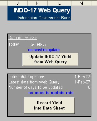
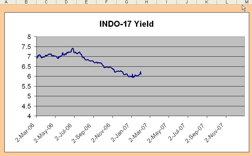
There are three sheets: INDO17, Data and Graph. "INDO17" is a sheet where the web query should go and where the two updating clicks are available. "Data" is a sheet where the bootstrapping process is running. "Graph" is only for visualisation.


Cell Naming


Cell naming is an important method as explained before in the previous post. There are several cells to be named in this worksheet and used for visual basic coding: INDO, INDOrow, INDOwebquery, nodays and updatelatestINDO.

To find which range is referred by a cell name, just go to the box on the top left, scroll the box and click the name. A range or cell will be shown.


  • INDO: a range as the destination for the updated rate from 2-Mar-06 to 31-Dec-10 in "Data" sheet (B5:B1263).
  • INDOrow: a cell showing a number of rows from 2-Mar-06 to the latest date has been updated in "Data" sheet (D3).
  • INDOwebquery: a range as the source of data captured via web query in "INDO17" sheet (A2:D21).
  • nodays: a cell showing a number of days need to be updated since the last updated date in "INDO17" sheet (M14).
  • updatelatestINDO: a cell showing the next date needs to be updated in "Data" sheet (G4).

Visual Basic Coding


Web Query Update
This code is for the first button "Update INDO-17 Yield from Web Query". The webpage source used for web query is the INDO-17 yield data provided in the Central Bank of Indonesia website.

The code:

Sub dailyINDO()

Application.OnTime Now + TimeValue("12:00:00"), "updateINDO"

End Sub

Sub updateINDO()

Sheets("INDO17").Activate
Range("a1").Select
Selection.QueryTable.Refresh BackgroundQuery:=True
dailyINDO

End Sub


Recording Data through Bootstrapping
This code is for the second button "Record Yield into Data Sheet". The code is quite complicated. However, if we can follow the logic and as referring to the range names, this is a piece of cake for us.

The code:

Sub recordINDO()

For j = 1 To Range("nodays")
For i = 1 To Range("nodays")

If Sheets("Data").Range("updatelatestINDO") = Range("INDOwebquery").Cells(i, 1) Then
Range("INDOwebquery").Cells(i, 4).Copy

r = Sheets("Data").Range("INDOrow") + 1

Sheets("Data").Range("INDO").Cells(r).PasteSpecial Paste:=xlPasteValues
Calculate
End If

Next i
Next j

Sheets("Data").Select

End Sub


The meaning of the above code is:

For the loops as many as the number of days needs to be updated, Excel will copy each yield in the web query sheet and paste into the data sheet on each corresponding date. Where the corresponding date is found by referring the number of rows from the first date to the latest updated date plus 1 day after.

Piece of cake, aye?


The "INDOrow"


It seems the key problem here is to find the number of "INDOrow", a cell showing a number of rows from 2-Mar-06 to the latest date has been updated in "Data" sheet (D3).

The way is using a MATCH function to calculate the number of rows from 2-Mar-06 to the latest date as this formulae:
=MATCH("latest date",C5:C498,0)

Where the "latest date" is found by tagging a note in the column C as the latest date using IF formulae: =IF(AND(the next yield=0, the current yield >0),"latest date","").


The "updatelatestINDO
"

This is a cell showing the next date needs to be updated in "Data" sheet (G4) that can be found easily using an INDEX function:

=INDEX($A$5:$A$498,INDOrow+1)


Recommendation and Notes

The title is for updating government bond yield, but the application can be also for updating other time series data such as foreign exchange rates or share prices.

I also open for any suggestions particularly for any more simple VBA codes.

Please let 2 days lag from Bank Indonesia website for current rate. It doesn't mean they are lazy to update, they just have a lot of other things to do.

More explanation about how to get data from the internet in Excel can be viewed here in Microsoft website.
Excel supports both reading and writing of XML. Complimenting this feature is the ability to create Web queries to XML files. You can create a Web query to any XML, but if you use the XML Spreadsheet schema, then you can preserve rich spreadsheet concepts like formulas.

Search This Blog

Powered by Blogger.